Getting started (for datasets with unaligned features)

Import the required packages:

import os
import sys
from pathlib import Path

import numpy as np
import pandas as pd
from matplotlib import pyplot as plt  # optional
import seaborn as sns  # optional

import scanpy as sc
from scipy import sparse

import networkx as nx
import torch

If you get trouble with installing CAME, you can download the source code from GitHub, and append the path to sys.path.

For example:

CAME_ROOT = Path('path/to/CAME')
sys.path.append(str(CAME_ROOT))

import came
from came import pipeline, pp, pl

ROOT = Path(".")  # set root

Using backend: pytorch

0 Load datasets

0.1 Load the example datasets

from came import load_example_data

example_data_dict = load_example_data()
print(example_data_dict.keys())

adatas = example_data_dict['adatas']
dsnames = example_data_dict['dataset_names']
df_varmap = example_data_dict['varmap']
df_varmap_1v1 = example_data_dict['varmap_1v1']

adata_raw1, adata_raw2 = adatas
key_class1 = key_class2 = example_data_dict['key_class']

# setting directory for results
time_tag = came.make_nowtime_tag()
resdir = ROOT /'_temp' / f'{dsnames}-{time_tag}'
figdir = resdir / 'figs'
came.check_dirs(figdir)  # check and make the directory

dict_keys(['adatas', 'varmap', 'varmap_1v1', 'dataset_names', 'key_class'])
a new directory made:
        _temp\('Baron_human', 'Baron_mouse')-(12-16 18.36.34)\figs

0.2 Load your own datasets

To load your own datasets, see the code example below:

# ========= customized paths ==========

dsnames = ('Baron_human', 'Baron_mouse')  # the dataset names, set by user
dsn1, dsn2 = dsnames

path_rawdata1 = CAME_ROOT / 'came/sample_data/raw-Baron_human.h5ad'
path_rawdata2 = CAME_ROOT / 'came/sample_data/raw-Baron_mouse.h5ad'

Path to homologous gene mappings, a dataframe with 2-columns, where the first column stores the reference genes and the second column stores the query ones.

Note that path_varmap_1v1 is optional (can be None). If not provided, the 1-to-1 homologous mappings will be inferred from the whole mappings.

path_varmap = CAME_ROOT / f'came/sample_data/gene_matches_human2mouse.csv'
path_varmap_1v1 = CAME_ROOT / f'came/sample_data/gene_matches_1v1_human2mouse.csv'

Load scRNA-seq datasets.

# ========= load data =========
df_varmap = pd.read_csv(path_varmap)
df_varmap_1v1 = pd.read_csv(path_varmap_1v1) if path_varmap_1v1 else came.pp.take_1v1_matches(df_varmap)

adata_raw1 = sc.read_h5ad(path_rawdata1)
adata_raw2 = sc.read_h5ad(path_rawdata2)
adatas = [adata_raw1, adata_raw2]

Sepcifiy the column names of the cell-type labels, where key_class1 is for reference data, and key_class2 is for query data. If there aren’t any cell-type or clustering labels for the query cells, you can set key_class=None.

key_class1 = 'cell_ontology_class'  # set by user
key_class2 = 'cell_ontology_class'  # set by user

Setting directory for results

time_tag = came.make_nowtime_tag()
resdir = ROOT /'_temp' / f'{dsnames}-{time_tag}'  # set by user
figdir = resdir / 'figs'
came.check_dirs(figdir)  # check and make the directory

Filtering genes (a preprocessing step, optional)

sc.pp.filter_genes(adata_raw1, min_cells=3)
sc.pp.filter_genes(adata_raw2, min_cells=3)

0.3 Inspect the compositions of different classes

# Inspect classes
if key_class2 is not None:
    group_counts_ori = pd.concat([
        pd.value_counts(adata_raw1.obs[key_class1]),
        pd.value_counts(adata_raw2.obs[key_class2]),
    ], axis=1, keys=dsnames)
else:
    group_counts_ori = pd.value_counts(adata_raw1.obs[key_class1])

group_counts_ori

	Baron_human	Baron_mouse
B cell	NaN	10.0
Schwann cell	13.0	6.0
T cell	7.0	7.0
endothelial cell	252.0	139.0
leukocyte	NaN	8.0
macrophage	55.0	36.0
mast cell	25.0	NaN
pancreatic A cell	2326.0	191.0
pancreatic D cell	601.0	218.0
pancreatic PP cell	255.0	41.0
pancreatic acinar cell	958.0	NaN
pancreatic ductal cell	1077.0	275.0
pancreatic epsilon cell	18.0	NaN
pancreatic stellate cell	457.0	61.0
type B pancreatic cell	2525.0	894.0

1 The default pipeline of CAME

Parameter settings.

# The numer of training epochs
# (a recommended setting is 200-400 for whole-graph training, and 80-200 for sub-graph training)
n_epochs = 300

# The training batch size
# When the GPU memory is limited, set 4096 or more if possible.
batch_size = None

# The number of epochs to skip for checkpoint backup
n_pass = 100

# Whether to use the single-cell networks
use_scnets = True

# The number of top DEGs to take as the node-features of each cells.
# You set it 70-100 for distant species pairs.
ntop_deg = 50

# The number of top DEGs to take as the graph nodes, which can be directly displayed on the UMAP plot.
ntop_deg_nodes = 50
# The source of the node genes; use both DEGs and HVGs by default
node_source = 'deg,hvg'

# Whether to take into account the non-1v1 variables as the node features.
keep_non1v1_feats = True

💡 An alternative choice for node genes is using only the DEGs:

>>> ntop_deg_nodes = 200
>>> node_source = 'deg'

⚠️ Note that if most of the homologies are non-1v1, better set keep_non1v1_feats as True, and increase the number of DEGs used as features ntop_deg

came_inputs, (adata1, adata2) = pipeline.preprocess_unaligned(
    adatas,
    key_class=key_class1,
    use_scnets=use_scnets,
    ntop_deg=ntop_deg,
    ntop_deg_nodes=ntop_deg_nodes,
    node_source=node_source,
)

outputs = pipeline.main_for_unaligned(
    **came_inputs,
    df_varmap=df_varmap,
    df_varmap_1v1=df_varmap_1v1,
    dataset_names=dsnames,
    key_class1=key_class1,
    key_class2=key_class2,
    do_normalize=True,
    keep_non1v1_feats=keep_non1v1_feats,
    n_epochs=n_epochs,
    resdir=resdir,
    n_pass=n_pass,
    batch_size=batch_size,
    plot_results=True,
)
dpair = outputs['dpair']
trainer = outputs['trainer']
h_dict = outputs['h_dict']
out_cell = outputs['out_cell']
predictor = outputs['predictor']


obs_ids1, obs_ids2 = dpair.obs_ids1, dpair.obs_ids2
obs = dpair.obs
classes = predictor.classes

[leiden] Time used:  0.2723 s
650 genes before taking unique
taking total of 501 unique differential expressed genes
400 genes before taking unique
taking total of 345 unique differential expressed genes
already exists:
        _temp\('Baron_human', 'Baron_mouse')-(12-16 18.36.34)\figs
already exists:
        _temp\('Baron_human', 'Baron_mouse')-(12-16 18.36.34)
[*] Setting dataset names:
        0-->Baron_human
        1-->Baron_mouse
[*] Setting aligned features for observation nodes (self._features)
[*] Setting un-aligned features (`self._ov_adjs`) for making links connecting observation and variable nodes
[*] Setting adjacent matrix connecting variables from these 2 datasets (`self._vv_adj`)
Index(['cell_ontology_class', 'cell_ontology_id', 'cell_type1', 'dataset_name',
       'donor', 'latent_1', 'latent_10', 'latent_2', 'latent_3', 'latent_4',
       'latent_5', 'latent_6', 'latent_7', 'latent_8', 'latent_9', 'library',
       'organ', 'organism', 'platform', 'tSNE1', 'tSNE2'],
      dtype='object')
Index(['cell_ontology_class', 'cell_ontology_id', 'cell_type1', 'dataset_name',
       'donor', 'latent_1', 'latent_10', 'latent_2', 'latent_3', 'latent_4',
       'latent_5', 'latent_6', 'latent_7', 'latent_8', 'latent_9', 'library',
       'organ', 'organism', 'platform', 'tSNE1', 'tSNE2', 'clust_lbs'],
      dtype='object')
-------------------- Summary of the DGL-Heterograph --------------------
Graph(num_nodes={'cell': 10455, 'gene': 6313},
      num_edges={('cell', 'express', 'gene'): 3793858, ('cell', 'self_loop_cell', 'cell'): 10455, ('cell', 'similar_to', 'cell'): 66764, ('gene', 'expressed_by', 'cell'): 3793858, ('gene', 'homolog_with', 'gene'): 11915},
      metagraph=[('cell', 'gene', 'express'), ('cell', 'cell', 'self_loop_cell'), ('cell', 'cell', 'similar_to'), ('gene', 'cell', 'expressed_by'), ('gene', 'gene', 'homolog_with')])
second-order connection: False
self-loops for observation-nodes: True
self-loops for variable-nodes: True
DataPair with 10455 obs- and 6313 var-nodes
obs1 x var1 (Baron_human): 8569 x 3332
obs2 x var2 (Baron_mouse): 1886 x 2981
Dimensions of the obs-node-features: 547
a new directory made:
        _temp\('Baron_human', 'Baron_mouse')-(12-16 18.36.34)\_models
main directory: _temp\('Baron_human', 'Baron_mouse')-(12-16 18.36.34)
model directory: _temp\('Baron_human', 'Baron_mouse')-(12-16 18.36.34)\_models
============== start training (device='cuda') ==============

C:\Users\Administrator\AppData\Roaming\Python\Python38\site-packages\torch\nn\modules\container.py:552: UserWarning: Setting attributes on ParameterDict is not supported.
  warnings.warn("Setting attributes on ParameterDict is not supported.")

Epoch 0000 | Train Acc: 0.0533 | Test: 0.0323 (max=0.0323) | AMI=-0.0000 | Time: 0.4114
Epoch 0005 | Train Acc: 0.2948 | Test: 0.4740 (max=0.4804) | AMI=0.0435 | Time: 0.1553
Epoch 0010 | Train Acc: 0.5011 | Test: 0.4899 (max=0.4899) | AMI=0.4180 | Time: 0.1315
Epoch 0015 | Train Acc: 0.4372 | Test: 0.6193 (max=0.6193) | AMI=0.4547 | Time: 0.1239
Epoch 0020 | Train Acc: 0.7186 | Test: 0.7174 (max=0.7174) | AMI=0.5456 | Time: 0.1194
Epoch 0025 | Train Acc: 0.7508 | Test: 0.7216 (max=0.7301) | AMI=0.5801 | Time: 0.1166
Epoch 0030 | Train Acc: 0.8419 | Test: 0.7937 (max=0.7937) | AMI=0.6283 | Time: 0.1149
Epoch 0035 | Train Acc: 0.8615 | Test: 0.8165 (max=0.8165) | AMI=0.6809 | Time: 0.1134
Epoch 0040 | Train Acc: 0.8743 | Test: 0.7773 (max=0.8165) | AMI=0.6177 | Time: 0.1124
Epoch 0045 | Train Acc: 0.8766 | Test: 0.7927 (max=0.8340) | AMI=0.6383 | Time: 0.1117
Epoch 0050 | Train Acc: 0.9152 | Test: 0.8208 (max=0.8340) | AMI=0.6644 | Time: 0.1110
Epoch 0055 | Train Acc: 0.9121 | Test: 0.8160 (max=0.8574) | AMI=0.6521 | Time: 0.1105
Epoch 0060 | Train Acc: 0.9420 | Test: 0.8627 (max=0.9067) | AMI=0.6900 | Time: 0.1101
Epoch 0065 | Train Acc: 0.9455 | Test: 0.8425 (max=0.9120) | AMI=0.6644 | Time: 0.1097
Epoch 0070 | Train Acc: 0.9531 | Test: 0.9067 (max=0.9120) | AMI=0.7347 | Time: 0.1096
Epoch 0075 | Train Acc: 0.9585 | Test: 0.9152 (max=0.9337) | AMI=0.7561 | Time: 0.1092
Epoch 0080 | Train Acc: 0.9639 | Test: 0.9268 (max=0.9337) | AMI=0.7646 | Time: 0.1091
Epoch 0085 | Train Acc: 0.9679 | Test: 0.9194 (max=0.9337) | AMI=0.7552 | Time: 0.1088
Epoch 0090 | Train Acc: 0.9722 | Test: 0.9290 (max=0.9358) | AMI=0.7685 | Time: 0.1088
Epoch 0095 | Train Acc: 0.9537 | Test: 0.9051 (max=0.9358) | AMI=0.7701 | Time: 0.1086
[current best] model weights backup
Epoch 0099 | Train Acc: 0.9673 | Test: 0.9099 (max=0.9358) | AMI=0.7497 | Time: 0.1088
[current best] model weights backup
Epoch 0100 | Train Acc: 0.9781 | Test: 0.9168 (max=0.9358) | AMI=0.7655 | Time: 0.1088
[current best] model weights backup
Epoch 0101 | Train Acc: 0.9718 | Test: 0.9300 (max=0.9358) | AMI=0.7725 | Time: 0.1091
[current best] model weights backup
Epoch 0104 | Train Acc: 0.9805 | Test: 0.9300 (max=0.9358) | AMI=0.7765 | Time: 0.1090
Epoch 0105 | Train Acc: 0.9798 | Test: 0.9231 (max=0.9358) | AMI=0.7519 | Time: 0.1090
[current best] model weights backup
Epoch 0106 | Train Acc: 0.9791 | Test: 0.9316 (max=0.9358) | AMI=0.7855 | Time: 0.1090
[current best] model weights backup
Epoch 0107 | Train Acc: 0.9807 | Test: 0.9300 (max=0.9358) | AMI=0.7866 | Time: 0.1090
[current best] model weights backup
Epoch 0109 | Train Acc: 0.9791 | Test: 0.9300 (max=0.9358) | AMI=0.7885 | Time: 0.1091
Epoch 0110 | Train Acc: 0.9793 | Test: 0.9210 (max=0.9358) | AMI=0.7842 | Time: 0.1090
Epoch 0115 | Train Acc: 0.9831 | Test: 0.9337 (max=0.9358) | AMI=0.7743 | Time: 0.1089
Epoch 0120 | Train Acc: 0.9835 | Test: 0.9295 (max=0.9358) | AMI=0.7763 | Time: 0.1088
[current best] model weights backup
Epoch 0123 | Train Acc: 0.9830 | Test: 0.9332 (max=0.9358) | AMI=0.8002 | Time: 0.1088
Epoch 0125 | Train Acc: 0.9828 | Test: 0.9014 (max=0.9358) | AMI=0.7312 | Time: 0.1088
model weights backup
Epoch 0129 | Train Acc: 0.9842 | Test: 0.9284 (max=0.9358) | AMI=0.7831 | Time: 0.1088
Epoch 0130 | Train Acc: 0.9821 | Test: 0.9364 (max=0.9364) | AMI=0.7930 | Time: 0.1088
Epoch 0135 | Train Acc: 0.9867 | Test: 0.9295 (max=0.9364) | AMI=0.7676 | Time: 0.1088
Epoch 0140 | Train Acc: 0.9837 | Test: 0.9252 (max=0.9401) | AMI=0.7799 | Time: 0.1087
Epoch 0145 | Train Acc: 0.9869 | Test: 0.9321 (max=0.9401) | AMI=0.7796 | Time: 0.1087
Epoch 0150 | Train Acc: 0.9882 | Test: 0.9247 (max=0.9401) | AMI=0.7689 | Time: 0.1086
[current best] model weights backup
Epoch 0152 | Train Acc: 0.9888 | Test: 0.9401 (max=0.9401) | AMI=0.8028 | Time: 0.1086
Epoch 0155 | Train Acc: 0.9893 | Test: 0.9374 (max=0.9401) | AMI=0.7850 | Time: 0.1086
Epoch 0160 | Train Acc: 0.9895 | Test: 0.9311 (max=0.9401) | AMI=0.7703 | Time: 0.1085
Epoch 0165 | Train Acc: 0.9894 | Test: 0.9337 (max=0.9401) | AMI=0.7990 | Time: 0.1084
[current best] model weights backup
Epoch 0167 | Train Acc: 0.9891 | Test: 0.9406 (max=0.9406) | AMI=0.8053 | Time: 0.1085
Epoch 0170 | Train Acc: 0.9895 | Test: 0.9369 (max=0.9406) | AMI=0.7956 | Time: 0.1085
model weights backup
Epoch 0172 | Train Acc: 0.9894 | Test: 0.9464 (max=0.9464) | AMI=0.7894 | Time: 0.1086
Epoch 0175 | Train Acc: 0.9897 | Test: 0.9427 (max=0.9464) | AMI=0.7962 | Time: 0.1085
[current best] model weights backup
Epoch 0178 | Train Acc: 0.9869 | Test: 0.9385 (max=0.9464) | AMI=0.8072 | Time: 0.1085
Epoch 0180 | Train Acc: 0.9893 | Test: 0.9417 (max=0.9464) | AMI=0.8058 | Time: 0.1085
Epoch 0185 | Train Acc: 0.9911 | Test: 0.9300 (max=0.9464) | AMI=0.7838 | Time: 0.1084
Epoch 0190 | Train Acc: 0.9908 | Test: 0.9364 (max=0.9464) | AMI=0.7876 | Time: 0.1084
Epoch 0195 | Train Acc: 0.9911 | Test: 0.9343 (max=0.9464) | AMI=0.7741 | Time: 0.1084
Epoch 0200 | Train Acc: 0.9895 | Test: 0.9369 (max=0.9464) | AMI=0.8005 | Time: 0.1083
Epoch 0205 | Train Acc: 0.9896 | Test: 0.9411 (max=0.9464) | AMI=0.7990 | Time: 0.1082
Epoch 0210 | Train Acc: 0.9907 | Test: 0.9183 (max=0.9464) | AMI=0.7845 | Time: 0.1082
model weights backup
Epoch 0215 | Train Acc: 0.9916 | Test: 0.9343 (max=0.9464) | AMI=0.7855 | Time: 0.1082
Epoch 0220 | Train Acc: 0.9918 | Test: 0.9390 (max=0.9475) | AMI=0.7800 | Time: 0.1082
Epoch 0225 | Train Acc: 0.9924 | Test: 0.9422 (max=0.9475) | AMI=0.7965 | Time: 0.1082
Epoch 0230 | Train Acc: 0.9932 | Test: 0.9443 (max=0.9475) | AMI=0.8003 | Time: 0.1082
[current best] model weights backup
Epoch 0235 | Train Acc: 0.9915 | Test: 0.9422 (max=0.9475) | AMI=0.8147 | Time: 0.1082
Epoch 0240 | Train Acc: 0.9900 | Test: 0.9284 (max=0.9475) | AMI=0.8111 | Time: 0.1081
Epoch 0245 | Train Acc: 0.9925 | Test: 0.9374 (max=0.9475) | AMI=0.7860 | Time: 0.1081
[current best] model weights backup
Epoch 0249 | Train Acc: 0.9914 | Test: 0.9475 (max=0.9475) | AMI=0.8221 | Time: 0.1081
Epoch 0250 | Train Acc: 0.9925 | Test: 0.9332 (max=0.9475) | AMI=0.7768 | Time: 0.1081
Epoch 0255 | Train Acc: 0.9936 | Test: 0.9385 (max=0.9475) | AMI=0.7926 | Time: 0.1080
model weights backup
Epoch 0258 | Train Acc: 0.9939 | Test: 0.9401 (max=0.9475) | AMI=0.7941 | Time: 0.1080
Epoch 0260 | Train Acc: 0.9946 | Test: 0.9449 (max=0.9475) | AMI=0.8087 | Time: 0.1080
Epoch 0265 | Train Acc: 0.9938 | Test: 0.9417 (max=0.9475) | AMI=0.8002 | Time: 0.1080
Epoch 0270 | Train Acc: 0.9935 | Test: 0.9390 (max=0.9491) | AMI=0.7870 | Time: 0.1079
[current best] model weights backup
Epoch 0275 | Train Acc: 0.9945 | Test: 0.9449 (max=0.9491) | AMI=0.8241 | Time: 0.1079
Epoch 0280 | Train Acc: 0.9951 | Test: 0.9454 (max=0.9491) | AMI=0.8111 | Time: 0.1079
Epoch 0285 | Train Acc: 0.9933 | Test: 0.9459 (max=0.9491) | AMI=0.8047 | Time: 0.1078
Epoch 0290 | Train Acc: 0.9954 | Test: 0.9486 (max=0.9491) | AMI=0.8155 | Time: 0.1078
Epoch 0295 | Train Acc: 0.9950 | Test: 0.9454 (max=0.9491) | AMI=0.8052 | Time: 0.1078
figure has been saved into:
        _temp\('Baron_human', 'Baron_mouse')-(12-16 18.36.34)\figs\cluster_index.png
states loaded from: _temp\('Baron_human', 'Baron_mouse')-(12-16 18.36.34)\_models\weights_epoch275.pt

C:\Users\Administrator\AppData\Roaming\Python\Python38\site-packages\torch\nn\modules\container.py:552: UserWarning: Setting attributes on ParameterDict is not supported.
  warnings.warn("Setting attributes on ParameterDict is not supported.")

object saved into:
         _temp\('Baron_human', 'Baron_mouse')-(12-16 18.36.34)\datapair_init.pickle
Re-order the rows
figure has been saved into:
        _temp\('Baron_human', 'Baron_mouse')-(12-16 18.36.34)\figs\contingency_matrix(acc94.5%).png
figure has been saved into:
        _temp\('Baron_human', 'Baron_mouse')-(12-16 18.36.34)\figs\contingency_matrix-train.png
figure has been saved into:
        _temp\('Baron_human', 'Baron_mouse')-(12-16 18.36.34)\figs\heatmap_probas.pdf

Load other checkpoint (optional)

You can load other model checkpoint if the default model is not satisfying.

For example, load the last checkpoint and compute the results of it:

outputs = pipeline.gather_came_results(
    dpair,
    trainer,
    classes=classes,
    keys=(key_class1, key_class2),
    keys_compare=(key_class1, key_class2),
    resdir=resdir,
    checkpoint='last',
    batch_size=None,
)

You can get all saved checkpoint numbers by:

came.get_checkpoint_list(resdir / '_models')

[100,
 101,
 104,
 106,
 107,
 109,
 123,
 129,
 152,
 167,
 172,
 178,
 215,
 235,
 249,
 258,
 275,
 299,
 99]

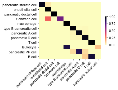
Plot the contingency matrix for query dataset

# contingency matrix for query dataset
y_true = obs['celltype'][obs_ids2].values
y_pred = obs['predicted'][obs_ids2].values

ax, contmat = pl.plot_contingency_mat(
    y_true, y_pred, norm_axis=1,
    order_rows=False, order_cols=False,
)
pl._save_with_adjust(ax.figure, figdir / 'contingency_mat.png')
ax.figure

figure has been saved into:
        _temp\('Baron_human', 'Baron_mouse')-(12-16 18.36.34)\figs\contingency_mat.png

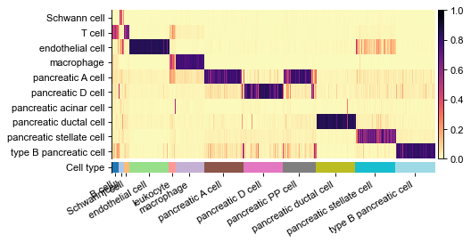
Plot heatmap of predicted probabilities

name_label = 'celltype'
cols_anno = ['celltype', 'predicted'][:]
df_probs = obs[list(classes)]


gs = pl.wrapper_heatmap_scores(
        df_probs.iloc[obs_ids2], obs.iloc[obs_ids2], ignore_index=True,
        col_label='celltype', col_pred='predicted',
        n_subsample=50,  # sampling 50 cells for each group
        cmap_heat='magma_r',
        fp=figdir / f'heatmap_probas.pdf'
    )

gs.figure

figure has been saved into:
        _temp\('Baron_human', 'Baron_mouse')-(12-16 18.36.34)\figs\heatmap_probas.pdf

2 Further analysis

By default, CAME will use the last layer of hidden states, as the embeddings, to produce cell- and gene-UMAP.

You can also load ALL of the model hidden states that have been seved during CAME’s default pipeline:

hidden_list = came.load_hidden_states(resdir / 'hidden_list.h5')
hidden_list  # a list of dicts
h_dict = hidden_list[-1]. # the last layer of hidden states

Make AnnData objects, storing only the CAME-embeddings and annotations, for cells and genes.

adt = pp.make_adata(h_dict['cell'], obs=dpair.obs, assparse=False, ignore_index=True)
gadt = pp.make_adata(h_dict['gene'], obs=dpair.var.iloc[:, :2], assparse=False, ignore_index=True)

# adt.write(resdir / 'adt_hidden_cell.h5ad')
# gadt.write_h5ad(resdir / 'adt_hidden_gene.h5ad')

adding columns to `adata.obs` (ignore_index=True):
original_name, dataset, REF, celltype, predicted, max_probs, is_right, pancreatic acinar cell, type B pancreatic cell, pancreatic D cell, pancreatic stellate cell, pancreatic ductal cell, pancreatic A cell, pancreatic epsilon cell, pancreatic PP cell, endothelial cell, macrophage, Schwann cell, mast cell, T cell, done!
adding columns to `adata.obs` (ignore_index=True):
name, dataset, done!

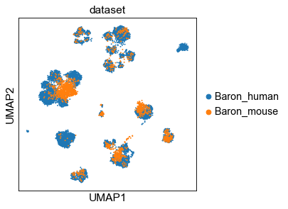
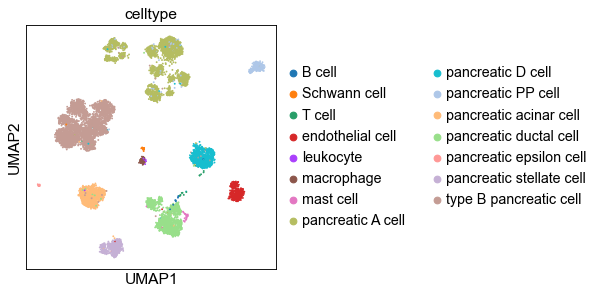
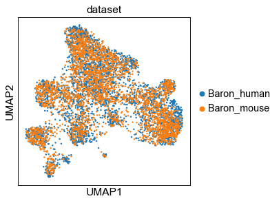
2.1 UMAP of cell embeddings

sc.set_figure_params(dpi_save=200)

sc.pp.neighbors(adt, n_neighbors=15, metric='cosine', use_rep='X')
sc.tl.umap(adt)
# sc.pl.umap(adt, color=['dataset', 'celltype'], ncols=1)

ftype = ['.svg', ''][1]
sc.pl.umap(adt, color='dataset', save=f'-dataset{ftype}')
sc.pl.umap(adt, color='celltype', save=f'-ctype{ftype}')

... storing 'dataset' as categorical
... storing 'REF' as categorical
... storing 'celltype' as categorical
... storing 'predicted' as categorical
WARNING: saving figure to file _temp\('Baron_human', 'Baron_mouse')-(12-16 18.36.34)\figs\umap-dataset.pdf

WARNING: saving figure to file _temp\('Baron_human', 'Baron_mouse')-(12-16 18.36.34)\figs\umap-ctype.pdf

Store UMAP coordinates:

obs_umap = adt.obsm['X_umap']
obs['UMAP1'] = obs_umap[:, 0]
obs['UMAP2'] = obs_umap[:, 1]
obs.to_csv(resdir / 'obs.csv')
adt.write(resdir / 'adt_hidden_cell.h5ad')

Setting UMAP to the original adata

adata1.obsm['X_umap'] = obs_umap[obs_ids1]
adata2.obsm['X_umap'] = obs_umap[obs_ids2]

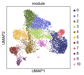
2.2 UMAP of genes

sc.pp.neighbors(gadt, n_neighbors=15, metric='cosine', use_rep='X')

# gadt = pp.make_adata(h_dict['gene'], obs=dpair.var.iloc[:, :2], assparse=False, ignore_index=True)
sc.tl.umap(gadt)
sc.pl.umap(gadt, color='dataset', )

... storing 'name' as categorical
... storing 'dataset' as categorical

# joint gene module extraction
sc.tl.leiden(gadt, resolution=.8, key_added='module')
sc.pl.umap(gadt, color='module', ncols=1, palette='tab20b')

# backup results is needed
# gadt.write(resdir / 'adt_hidden_gene.h5ad')

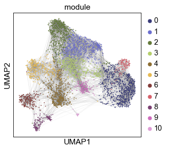
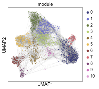
Visualize gene UMAPs:

# gadt.obs_names = gadt.obs_names.astype(str)
gadt1, gadt2 = pp.bisplit_adata(gadt, 'dataset', dsnames[0], reset_index_by='name')

color_by = 'module'
palette = 'tab20b'
sc.pl.umap(gadt1, color=color_by, s=10, edges=True, edges_width=0.05,
           palette=palette,
           save=f'_{color_by}-{dsnames[0]}')
sc.pl.umap(gadt2, color=color_by, s=10, edges=True, edges_width=0.05,
           palette=palette,
           save=f'_{color_by}-{dsnames[0]}')

WARNING: saving figure to file _temp\('Baron_human', 'Baron_mouse')-(12-16 18.36.34)\figs\umap_module-Baron_human.pdf

WARNING: saving figure to file _temp\('Baron_human', 'Baron_mouse')-(12-16 18.36.34)\figs\umap_module-Baron_human.pdf

Compute the link-weights (embedding similarity) between homologous gene pairs:

df_var_links = came.weight_linked_vars(
    gadt.X, dpair._vv_adj, names=dpair.get_vnode_names(),
    matric='cosine', index_names=dsnames,
)

gadt1.write(resdir / 'adt_hidden_gene1.h5ad')
gadt2.write(resdir / 'adt_hidden_gene2.h5ad')

2.3 Gene-expression-profiles (for each cell type) on gene UMAP

Compute average expressions for each cell type.

# averaged expressions
avg_expr1 = pp.group_mean_adata(
    adatas[0], groupby=key_class1,
    features=dpair.vnode_names1, use_raw=True)
avg_expr2 = pp.group_mean_adata(
    adatas[1], groupby=key_class2 if key_class2 else 'predicted',
    features=dpair.vnode_names2, use_raw=True)

Computing averages grouped by cell_ontology_class
Computing averages grouped by cell_ontology_class

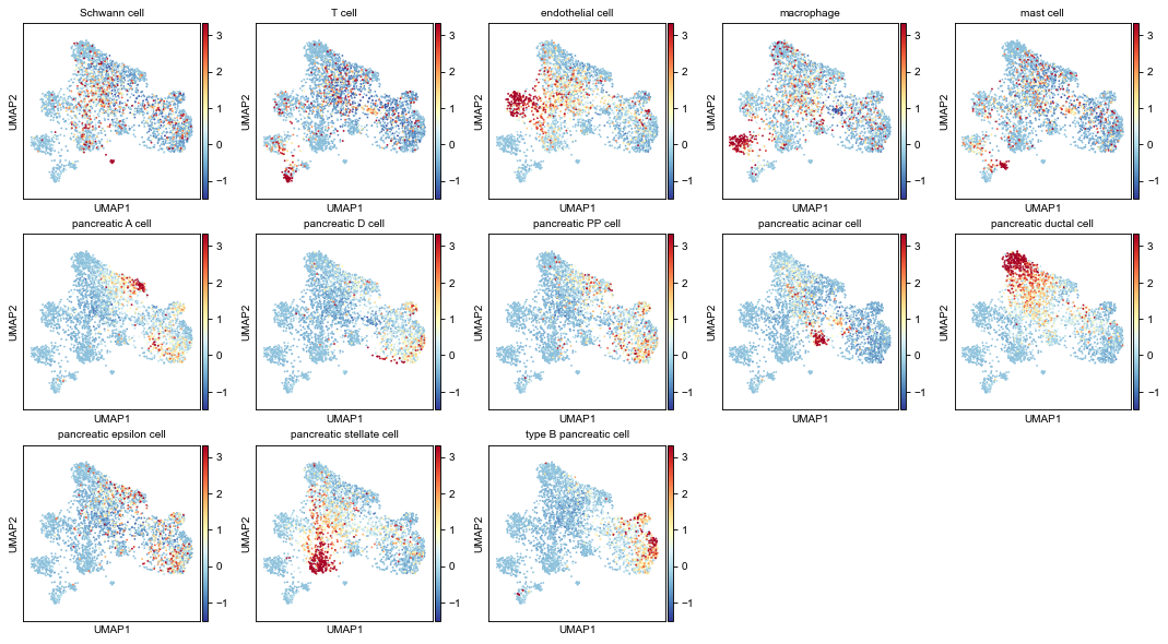
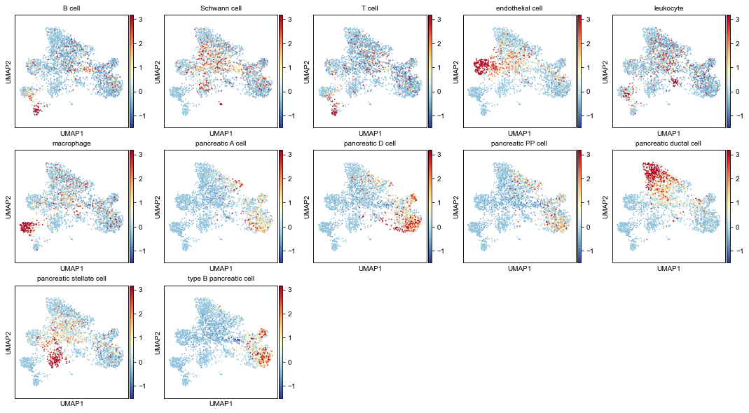
plot cell type gene-profiles (plot all the cell types) on UMAP

plkwds = dict(cmap='RdYlBu_r', vmax=2.5, vmin=-1.5, do_zscore=True,
              axscale=3, ncols=5, with_cbar=True)

fig1, axs1 = pl.adata_embed_with_values(
    gadt1, avg_expr1,
    fp=figdir / f'umap_exprAvgs-{dsnames[0]}-all.png',
    **plkwds)
fig2, axs2 = pl.adata_embed_with_values(
    gadt2, avg_expr2,
    fp=figdir / f'umap_exprAvgs-{dsnames[1]}-all.png',
    **plkwds)

figure has been saved into:
        _temp\('Baron_human', 'Baron_mouse')-(12-16 18.36.34)\figs\umap_exprAvgs-Baron_human-all.png
figure has been saved into:
        _temp\('Baron_human', 'Baron_mouse')-(12-16 18.36.34)\figs\umap_exprAvgs-Baron_mouse-all.png

fig1

fig2

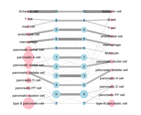
2.4 Abstracted graph

norm_ov = ['max', 'zs', None][1]
cut_ov = 0.

groupby_var = 'module'
obs_labels1, obs_labels2 = adt.obs['celltype'][dpair.obs_ids1], \
                           adt.obs['celltype'][dpair.obs_ids2]
var_labels1, var_labels2 = gadt1.obs[groupby_var], gadt2.obs[groupby_var]

sp1, sp2 = 'human', 'mouse'
g = came.make_abstracted_graph(
    obs_labels1, obs_labels2,
    var_labels1, var_labels2,
    avg_expr1, avg_expr2,
    df_var_links,
    tags_obs=(f'{sp1} ', f'{sp2} '),
    tags_var=(f'{sp1} module ', f'{sp2} module '),
    cut_ov=cut_ov,
    norm_mtd_ov=norm_ov,
)

3332 2981
Edges with weights lower than 0 were cut out.
Edges with weights lower than 0 were cut out.
2801
2801 2801
---> aggregating edges...
unique labels of rows: ['5' '1' '2' '4' '6' '0' '9' '3' '7' '8' '10']
unique labels of columns: ['6' '2' '0' '7' '8' '9' '3' '5' '1' '4' '10']
grouping elements (edges)
shape of the one-hot-labels: (3332, 11) (2981, 11)
Re-order the rows
Re-order the columns
Re-order the columns
Re-order the columns
2801
2801 2801
---> aggregating edges...
unique labels of rows: ['5' '1' '2' '4' '6' '0' '9' '3' '7' '8' '10']
unique labels of columns: ['6' '2' '0' '7' '8' '9' '3' '5' '1' '4' '10']
grouping elements (edges)
shape of the one-hot-labels: (3332, 11) (2981, 11)

''' visualization '''
fp_abs = figdir / f'abstracted_graph-{groupby_var}-cut{cut_ov}-{norm_ov}.pdf'
ax = pl.plot_multipartite_graph(
    g, edge_scale=10,
    figsize=(9, 7.5), alpha=0.5, fp=fp_abs)  # nodelist=nodelist,

ax.figure

[13, 11, 11, 12]
figure has been saved into:
        _temp\('Baron_human', 'Baron_mouse')-(12-16 18.36.34)\figs\abstracted_graph-module-cut0.0-zs.pdf

# save abstracted-graph object
came.save_pickle(g, resdir / 'abs_graph.pickle')

object saved into:
         _temp\('Baron_human', 'Baron_mouse')-(12-16 18.36.34)\abs_graph.pickle