Getting started (for datasets with aligned features)

Import the required packages:

import os
import sys
from pathlib import Path

import numpy as np
import pandas as pd
from matplotlib import pyplot as plt  # optional
import seaborn as sns  # optional

import scanpy as sc
from scipy import sparse

import networkx as nx
import torch

If you get trouble with installing CAME, you can download the source code from GitHub, and append the path to sys.path. For example:

CAME_ROOT = Path('path/to/CAME')
sys.path.append(str(CAME_ROOT))

import came
from came import pipeline, pp, pl

ROOT = Path(".")  # set root

Using backend: pytorch

0 Load datasets

0.1 Load the example datasets

from came import load_example_data

example_data_dict = load_example_data()
print(example_data_dict.keys())

adatas = example_data_dict['adatas']
dsnames = example_data_dict['dataset_names']

adata_raw1, adata_raw2 = adatas
key_class1 = key_class2 = example_data_dict['key_class']

df_varmap_1v1 = example_data_dict['varmap_1v1']   # set as None if NOT cross species

# setting directory for results
time_tag = came.make_nowtime_tag()
resdir = ROOT /'_temp' / f'{dsnames}-{time_tag}'
figdir = resdir / 'figs'
came.check_dirs(figdir)  # check and make the directory

dict_keys(['adatas', 'varmap', 'varmap_1v1', 'dataset_names', 'key_class'])
a new directory made:
        _temp\('Baron_human', 'Baron_mouse')-(12-16 18.13.20)\figs

0.2 Load your own datasets

To load your own datasets, see the code example below:

# ========= customized paths ==========

dsnames = ('Baron_human', 'Baron_mouse')  # the dataset names, set by user
dsn1, dsn2 = dsnames

path_rawdata1 = CAME_ROOT / 'came/sample_data/raw-Baron_human.h5ad'
path_rawdata2 = CAME_ROOT / 'came/sample_data/raw-Baron_mouse.h5ad'
path_varmap_1v1 = CAME_ROOT / f'came/sample_data/gene_matches_1v1_human2mouse.csv'

Load scRNA-seq datasets.

# ========= load data =========
df_varmap = pd.read_csv(path_varmap)
df_varmap_1v1 = pd.read_csv(path_varmap_1v1) if path_varmap_1v1 else came.pp.take_1v1_matches(df_varmap)

adata_raw1 = sc.read_h5ad(path_rawdata1)
adata_raw2 = sc.read_h5ad(path_rawdata2)
adatas = [adata_raw1, adata_raw2]

Sepcifiy the column names of the cell-type labels, where key_class1 is for reference data, and key_class2 is for query data. If there aren’t any cell-type or clustering labels for the query cells, you can set key_class=None.

key_class1 = 'cell_ontology_class'  # set by user
key_class2 = 'cell_ontology_class'  # set by user

Setting directory for results

time_tag = came.make_nowtime_tag()
resdir = ROOT /'_temp' / f'{dsnames}-{time_tag}'  # set by user
figdir = resdir / 'figs'
came.check_dirs(figdir)  # check and make the directory

Filtering genes (a preprocessing step, optional)

sc.pp.filter_genes(adata_raw1, min_cells=3)
sc.pp.filter_genes(adata_raw2, min_cells=3)

0.3 Inspect the compositions of different classes

# Inspect classes
if key_class2 is not None:
    group_counts_ori = pd.concat([
        pd.value_counts(adata_raw1.obs[key_class1]),
        pd.value_counts(adata_raw2.obs[key_class2]),
    ], axis=1)
else:
    group_counts_ori = pd.value_counts(adata_raw1.obs[key_class1])


group_counts_ori

	cell_ontology_class	cell_ontology_class
B cell	NaN	10.0
Schwann cell	13.0	6.0
T cell	7.0	7.0
endothelial cell	252.0	139.0
leukocyte	NaN	8.0
macrophage	55.0	36.0
mast cell	25.0	NaN
pancreatic A cell	2326.0	191.0
pancreatic D cell	601.0	218.0
pancreatic PP cell	255.0	41.0
pancreatic acinar cell	958.0	NaN
pancreatic ductal cell	1077.0	275.0
pancreatic epsilon cell	18.0	NaN
pancreatic stellate cell	457.0	61.0
type B pancreatic cell	2525.0	894.0

1 The default pipeline of CAME

Parameter setting:

# the numer of training epochs
# (a recommended setting is 200-400 for whole-graph training, and 80-200 for sub-graph training)
n_epochs = 300

# the training batch size
# When the GPU memory is limited, set 1024 or more if possible.
batch_size = None

# the number of epochs to skip for checkpoint backup
n_pass = 100

# whether to use the single-cell networks
use_scnets = True

# node genes, use both the DEGs and HVGs by default
node_source = 'deg,hvg'
ntop_deg = 50

came_inputs, (adata1, adata2) = pipeline.preprocess_aligned(
    adatas,
    key_class=key_class1,
    use_scnets=use_scnets,
    ntop_deg=ntop_deg,
    node_source=node_source,
    df_varmap_1v1=df_varmap_1v1,  # set as None if NOT cross species
)

outputs = pipeline.main_for_aligned(
    **came_inputs,
    dataset_names=dsnames,
    key_class1=key_class1,
    key_class2=key_class2,
    do_normalize=True,
    n_epochs=n_epochs,
    resdir=resdir,
    n_pass=n_pass,
    batch_size=batch_size,
    plot_results=True,
)
dpair = outputs['dpair']
trainer = outputs['trainer']
h_dict = outputs['h_dict']
out_cell = outputs['out_cell']
predictor = outputs['predictor']

obs_ids1, obs_ids2 = dpair.obs_ids1, dpair.obs_ids2
obs = dpair.obs
classes = predictor.classes

[leiden] Time used:  0.2753 s
650 genes before taking unique
taking total of 494 unique differential expressed genes
450 genes before taking unique
taking total of 369 unique differential expressed genes
already exists:
        _temp\('Baron_human', 'Baron_mouse')-(12-16 18.13.20)\figs
already exists:
        _temp\('Baron_human', 'Baron_mouse')-(12-16 18.13.20)
[*] Setting dataset names:
        0-->Baron_human
        1-->Baron_mouse
[*] Setting aligned features for observation nodes (self._features)
[*] Setting observation-by-variable adjacent matrices (`self._ov_adjs`) for making merged graph adjacent matrix of observation and variable nodes
-------------------- Summary of the DGL-Heterograph --------------------
Graph(num_nodes={'cell': 10455, 'gene': 3343},
      num_edges={('cell', 'express', 'gene'): 4257363, ('cell', 'self_loop_cell', 'cell'): 10455, ('cell', 'similar_to', 'cell'): 65800, ('gene', 'expressed_by', 'cell'): 4257363, ('gene', 'self_loop_gene', 'gene'): 3343},
      metagraph=[('cell', 'gene', 'express'), ('cell', 'cell', 'self_loop_cell'), ('cell', 'cell', 'similar_to'), ('gene', 'cell', 'expressed_by'), ('gene', 'gene', 'self_loop_gene')])
self-loops for observation-nodes: True
self-loops for variable-nodes: True
AlignedDataPair with 10455 obs- and 3343 var-nodes
n_obs1 (Baron_human): 8569
n_obs2 (Baron_mouse): 1886
Dimensions of the obs-node-features: 702
a new directory made:
        _temp\('Baron_human', 'Baron_mouse')-(12-16 18.13.20)\_models
main directory: _temp\('Baron_human', 'Baron_mouse')-(12-16 18.13.20)
model directory: _temp\('Baron_human', 'Baron_mouse')-(12-16 18.13.20)\_models
============== start training (device='cuda') ==============

C:\Users\Administrator\AppData\Roaming\Python\Python38\site-packages\torch\nn\modules\container.py:552: UserWarning: Setting attributes on ParameterDict is not supported.
  warnings.warn("Setting attributes on ParameterDict is not supported.")

Epoch 0000 | Train Acc: 0.1117 | Test: 0.0021 (max=0.0021) | AMI=0.0075 | Time: 0.4064
Epoch 0005 | Train Acc: 0.4159 | Test: 0.2519 (max=0.2519) | AMI=0.2858 | Time: 0.1625
Epoch 0010 | Train Acc: 0.3867 | Test: 0.5403 (max=0.5403) | AMI=0.1705 | Time: 0.1396
Epoch 0015 | Train Acc: 0.7065 | Test: 0.4592 (max=0.6013) | AMI=0.3634 | Time: 0.1313
Epoch 0020 | Train Acc: 0.7971 | Test: 0.6092 (max=0.6310) | AMI=0.4382 | Time: 0.1269
Epoch 0025 | Train Acc: 0.8147 | Test: 0.7386 (max=0.7386) | AMI=0.5266 | Time: 0.1244
Epoch 0030 | Train Acc: 0.8661 | Test: 0.7476 (max=0.7476) | AMI=0.5507 | Time: 0.1229
Epoch 0035 | Train Acc: 0.8759 | Test: 0.7359 (max=0.7720) | AMI=0.5480 | Time: 0.1218
Epoch 0040 | Train Acc: 0.9209 | Test: 0.7736 (max=0.7736) | AMI=0.5692 | Time: 0.1207
Epoch 0045 | Train Acc: 0.9447 | Test: 0.7667 (max=0.7842) | AMI=0.5618 | Time: 0.1200
Epoch 0050 | Train Acc: 0.9632 | Test: 0.8033 (max=0.8043) | AMI=0.6154 | Time: 0.1194
Epoch 0055 | Train Acc: 0.9725 | Test: 0.7789 (max=0.8420) | AMI=0.6129 | Time: 0.1189
Epoch 0060 | Train Acc: 0.9748 | Test: 0.8028 (max=0.8537) | AMI=0.6226 | Time: 0.1185
Epoch 0065 | Train Acc: 0.9757 | Test: 0.8441 (max=0.8600) | AMI=0.6777 | Time: 0.1182
Epoch 0070 | Train Acc: 0.9786 | Test: 0.8452 (max=0.8802) | AMI=0.6295 | Time: 0.1180
Epoch 0075 | Train Acc: 0.9800 | Test: 0.8834 (max=0.8834) | AMI=0.6664 | Time: 0.1178
Epoch 0080 | Train Acc: 0.9823 | Test: 0.8621 (max=0.8834) | AMI=0.6479 | Time: 0.1176
Epoch 0085 | Train Acc: 0.9828 | Test: 0.8706 (max=0.8834) | AMI=0.6571 | Time: 0.1175
Epoch 0090 | Train Acc: 0.9858 | Test: 0.8621 (max=0.8834) | AMI=0.6353 | Time: 0.1174
Epoch 0095 | Train Acc: 0.9875 | Test: 0.8754 (max=0.8913) | AMI=0.6688 | Time: 0.1173
[current best] model weights backup
Epoch 0099 | Train Acc: 0.9876 | Test: 0.8770 (max=0.8913) | AMI=0.6630 | Time: 0.1173
[current best] model weights backup
Epoch 0100 | Train Acc: 0.9872 | Test: 0.8871 (max=0.8913) | AMI=0.6810 | Time: 0.1173
[current best] model weights backup
Epoch 0101 | Train Acc: 0.9879 | Test: 0.8913 (max=0.8913) | AMI=0.6932 | Time: 0.1174
Epoch 0105 | Train Acc: 0.9874 | Test: 0.8807 (max=0.8913) | AMI=0.6850 | Time: 0.1173
[current best] model weights backup
Epoch 0106 | Train Acc: 0.9870 | Test: 0.8902 (max=0.8913) | AMI=0.6961 | Time: 0.1174
[current best] model weights backup
Epoch 0110 | Train Acc: 0.9887 | Test: 0.8945 (max=0.8945) | AMI=0.6973 | Time: 0.1174
[current best] model weights backup
Epoch 0114 | Train Acc: 0.9888 | Test: 0.9062 (max=0.9062) | AMI=0.7225 | Time: 0.1174
Epoch 0115 | Train Acc: 0.9898 | Test: 0.8621 (max=0.9062) | AMI=0.6486 | Time: 0.1174
Epoch 0120 | Train Acc: 0.9898 | Test: 0.8897 (max=0.9062) | AMI=0.6883 | Time: 0.1172
Epoch 0125 | Train Acc: 0.9916 | Test: 0.8908 (max=0.9104) | AMI=0.6930 | Time: 0.1172
model weights backup
Epoch 0129 | Train Acc: 0.9909 | Test: 0.8765 (max=0.9104) | AMI=0.6649 | Time: 0.1171
Epoch 0130 | Train Acc: 0.9916 | Test: 0.8955 (max=0.9104) | AMI=0.6903 | Time: 0.1171
Epoch 0135 | Train Acc: 0.9914 | Test: 0.9062 (max=0.9104) | AMI=0.7135 | Time: 0.1170
Epoch 0140 | Train Acc: 0.9926 | Test: 0.8839 (max=0.9130) | AMI=0.6769 | Time: 0.1169
[current best] model weights backup
Epoch 0142 | Train Acc: 0.9886 | Test: 0.8987 (max=0.9130) | AMI=0.7245 | Time: 0.1169
Epoch 0145 | Train Acc: 0.9896 | Test: 0.8918 (max=0.9130) | AMI=0.6879 | Time: 0.1168
[current best] model weights backup
Epoch 0147 | Train Acc: 0.9929 | Test: 0.9120 (max=0.9130) | AMI=0.7280 | Time: 0.1168
Epoch 0150 | Train Acc: 0.9925 | Test: 0.9003 (max=0.9130) | AMI=0.7154 | Time: 0.1167
[current best] model weights backup
Epoch 0155 | Train Acc: 0.9929 | Test: 0.9311 (max=0.9311) | AMI=0.7515 | Time: 0.1168
Epoch 0160 | Train Acc: 0.9933 | Test: 0.9268 (max=0.9311) | AMI=0.7474 | Time: 0.1167
Epoch 0165 | Train Acc: 0.9939 | Test: 0.9136 (max=0.9311) | AMI=0.7268 | Time: 0.1167
Epoch 0170 | Train Acc: 0.9932 | Test: 0.9051 (max=0.9311) | AMI=0.7153 | Time: 0.1166
[current best] model weights backup
Epoch 0171 | Train Acc: 0.9935 | Test: 0.9290 (max=0.9311) | AMI=0.7526 | Time: 0.1166
[current best] model weights backup
Epoch 0172 | Train Acc: 0.9935 | Test: 0.9327 (max=0.9327) | AMI=0.7537 | Time: 0.1166
Epoch 0175 | Train Acc: 0.9924 | Test: 0.9252 (max=0.9327) | AMI=0.7476 | Time: 0.1166
Epoch 0180 | Train Acc: 0.9932 | Test: 0.8977 (max=0.9327) | AMI=0.7001 | Time: 0.1165
[current best] model weights backup
Epoch 0181 | Train Acc: 0.9937 | Test: 0.9300 (max=0.9327) | AMI=0.7598 | Time: 0.1166
[current best] model weights backup
Epoch 0183 | Train Acc: 0.9930 | Test: 0.9305 (max=0.9327) | AMI=0.7642 | Time: 0.1166
Epoch 0185 | Train Acc: 0.9928 | Test: 0.9247 (max=0.9327) | AMI=0.7592 | Time: 0.1165
Epoch 0190 | Train Acc: 0.9939 | Test: 0.9279 (max=0.9327) | AMI=0.7348 | Time: 0.1165
[current best] model weights backup
Epoch 0191 | Train Acc: 0.9937 | Test: 0.9417 (max=0.9417) | AMI=0.7866 | Time: 0.1165
Epoch 0195 | Train Acc: 0.9946 | Test: 0.9343 (max=0.9417) | AMI=0.7492 | Time: 0.1165
Epoch 0200 | Train Acc: 0.9952 | Test: 0.9464 (max=0.9464) | AMI=0.7792 | Time: 0.1165
Epoch 0205 | Train Acc: 0.9950 | Test: 0.9247 (max=0.9464) | AMI=0.7457 | Time: 0.1165
[current best] model weights backup
Epoch 0207 | Train Acc: 0.9945 | Test: 0.9464 (max=0.9464) | AMI=0.7906 | Time: 0.1166
Epoch 0210 | Train Acc: 0.9949 | Test: 0.9321 (max=0.9464) | AMI=0.7565 | Time: 0.1165
model weights backup
Epoch 0215 | Train Acc: 0.9954 | Test: 0.9390 (max=0.9491) | AMI=0.7636 | Time: 0.1165
[current best] model weights backup
Epoch 0220 | Train Acc: 0.9949 | Test: 0.9486 (max=0.9491) | AMI=0.7920 | Time: 0.1165
Epoch 0225 | Train Acc: 0.9956 | Test: 0.9496 (max=0.9496) | AMI=0.7870 | Time: 0.1165
[current best] model weights backup
Epoch 0229 | Train Acc: 0.9954 | Test: 0.9433 (max=0.9496) | AMI=0.7942 | Time: 0.1164
Epoch 0230 | Train Acc: 0.9946 | Test: 0.9343 (max=0.9496) | AMI=0.7742 | Time: 0.1164
Epoch 0235 | Train Acc: 0.9945 | Test: 0.9104 (max=0.9496) | AMI=0.7167 | Time: 0.1164
[current best] model weights backup
Epoch 0239 | Train Acc: 0.9954 | Test: 0.9517 (max=0.9517) | AMI=0.8013 | Time: 0.1164
Epoch 0240 | Train Acc: 0.9956 | Test: 0.9443 (max=0.9517) | AMI=0.7786 | Time: 0.1164
Epoch 0245 | Train Acc: 0.9964 | Test: 0.9470 (max=0.9517) | AMI=0.7858 | Time: 0.1164
Epoch 0250 | Train Acc: 0.9964 | Test: 0.9321 (max=0.9517) | AMI=0.7595 | Time: 0.1164
[current best] model weights backup
Epoch 0252 | Train Acc: 0.9967 | Test: 0.9491 (max=0.9517) | AMI=0.8026 | Time: 0.1164
Epoch 0255 | Train Acc: 0.9965 | Test: 0.9422 (max=0.9517) | AMI=0.7758 | Time: 0.1164
model weights backup
Epoch 0258 | Train Acc: 0.9965 | Test: 0.9475 (max=0.9517) | AMI=0.7836 | Time: 0.1164
Epoch 0260 | Train Acc: 0.9972 | Test: 0.9491 (max=0.9517) | AMI=0.7829 | Time: 0.1164
Epoch 0265 | Train Acc: 0.9973 | Test: 0.9480 (max=0.9517) | AMI=0.7765 | Time: 0.1164
Epoch 0270 | Train Acc: 0.9968 | Test: 0.9470 (max=0.9517) | AMI=0.7744 | Time: 0.1163
[current best] model weights backup
Epoch 0274 | Train Acc: 0.9963 | Test: 0.9571 (max=0.9571) | AMI=0.8026 | Time: 0.1163
Epoch 0275 | Train Acc: 0.9974 | Test: 0.9517 (max=0.9571) | AMI=0.7910 | Time: 0.1163
Epoch 0280 | Train Acc: 0.9972 | Test: 0.9533 (max=0.9571) | AMI=0.7987 | Time: 0.1163
Epoch 0285 | Train Acc: 0.9960 | Test: 0.9517 (max=0.9571) | AMI=0.7967 | Time: 0.1163
Epoch 0290 | Train Acc: 0.9967 | Test: 0.9396 (max=0.9571) | AMI=0.7713 | Time: 0.1163
[current best] model weights backup
Epoch 0291 | Train Acc: 0.9971 | Test: 0.9496 (max=0.9571) | AMI=0.8040 | Time: 0.1163
Epoch 0295 | Train Acc: 0.9972 | Test: 0.9459 (max=0.9571) | AMI=0.8006 | Time: 0.1162
figure has been saved into:
        _temp\('Baron_human', 'Baron_mouse')-(12-16 18.13.20)\figs\cluster_index.png
states loaded from: _temp\('Baron_human', 'Baron_mouse')-(12-16 18.13.20)\_models\weights_epoch291.pt

C:\Users\Administrator\AppData\Roaming\Python\Python38\site-packages\torch\nn\modules\container.py:552: UserWarning: Setting attributes on ParameterDict is not supported.
  warnings.warn("Setting attributes on ParameterDict is not supported.")

object saved into:
         _temp\('Baron_human', 'Baron_mouse')-(12-16 18.13.20)\datapair_init.pickle
Re-order the rows
figure has been saved into:
        _temp\('Baron_human', 'Baron_mouse')-(12-16 18.13.20)\figs\contingency_matrix(acc95.0%).png
figure has been saved into:
        _temp\('Baron_human', 'Baron_mouse')-(12-16 18.13.20)\figs\contingency_matrix-train.png
figure has been saved into:
        _temp\('Baron_human', 'Baron_mouse')-(12-16 18.13.20)\figs\heatmap_probas.pdf

Load other checkpoint (optional)

You can load other model checkpoint if the default model is not satisfying.

For example, load the last checkpoint and compute the results of it:

outputs = pipeline.gather_came_results(
    dpair,
    trainer,
    classes=classes,
    keys=(key_class1, key_class2),
    keys_compare=(key_class1, key_class2),
    resdir=resdir,
    checkpoint='last',
    batch_size=None,
)

You can get all saved checkpoint numbers by:

came.get_checkpoint_list(resdir / '_models')

[100,
 101,
 106,
 110,
 114,
 129,
 142,
 147,
 155,
 171,
 172,
 181,
 183,
 191,
 207,
 215,
 220,
 229,
 239,
 252,
 258,
 274,
 291,
 299,
 99]

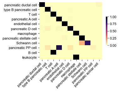
Plot the contingency matrix for query dataset

# contingency matrix for query dataset
y_true = obs['celltype'][obs_ids2].values
y_pred = obs['predicted'][obs_ids2].values

ax, contmat = pl.plot_contingency_mat(
    y_true, y_pred, norm_axis=1,
    order_rows=False, order_cols=False,
)
pl._save_with_adjust(ax.figure, figdir / 'contingency_mat.png')
ax.figure

figure has been saved into:
        _temp\('Baron_human', 'Baron_mouse')-(12-16 18.13.20)\figs\contingency_mat.png

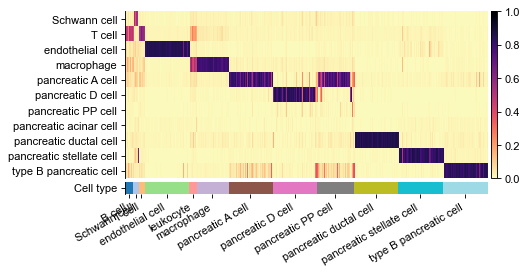
Plot heatmap of predicted probabilities

name_label = 'celltype'
cols_anno = ['celltype', 'predicted'][:]
df_probs = obs[list(classes)]


gs = pl.wrapper_heatmap_scores(
        df_probs.iloc[obs_ids2], obs.iloc[obs_ids2], ignore_index=True,
        col_label='celltype', col_pred='predicted',
        n_subsample=50,
        cmap_heat='magma_r',  # if prob_func == 'softmax' else 'RdBu_r'
        fp=figdir / f'heatmap_probas.pdf'
    )

gs.figure

figure has been saved into:
        _temp\('Baron_human', 'Baron_mouse')-(12-16 18.13.20)\figs\heatmap_probas.pdf

2 Further analysis

By default, CAME will use the last layer of hidden states, as the embeddings, to produce cell- and gene-UMAP.

You can also load ALL of the model hidden states that have been seved during CAME’s default pipeline:

hidden_list = came.load_hidden_states(resdir / 'hidden_list.h5')
hidden_list  # a list of dicts
h_dict = hidden_list[-1]. # the last layer of hidden states

Make AnnData objects, storing only the CAME-embeddings and annotations, for cells and genes.

adt = pp.make_adata(h_dict['cell'], obs=dpair.obs, assparse=False, ignore_index=True)
gadt = pp.make_adata(h_dict['gene'], obs=dpair.var.iloc[:, :2], assparse=False, ignore_index=True)

# adt.write(resdir / 'adt_hidden_cell.h5ad')
# gadt.write_h5ad(resdir / 'adt_hidden_gene.h5ad')

adding columns to `adata.obs` (ignore_index=True):
original_name, dataset, REF, celltype, predicted, max_probs, is_right, pancreatic acinar cell, type B pancreatic cell, pancreatic D cell, pancreatic stellate cell, pancreatic ductal cell, pancreatic A cell, pancreatic epsilon cell, pancreatic PP cell, endothelial cell, macrophage, Schwann cell, mast cell, T cell, done!
adding columns to `adata.obs` (ignore_index=True):
name, done!

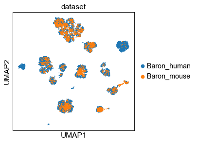
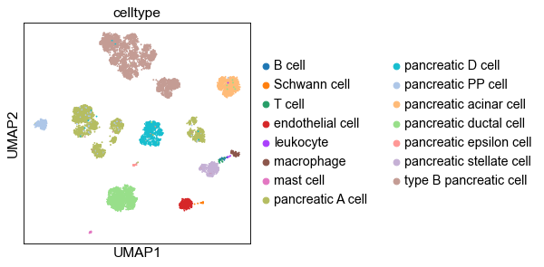
UMAP of cell embeddings

sc.set_figure_params(dpi_save=200)

sc.pp.neighbors(adt, n_neighbors=15, metric='cosine', use_rep='X')
sc.tl.umap(adt)
# sc.pl.umap(adt, color=['dataset', 'celltype'], ncols=1)

ftype = ['.svg', ''][1]
sc.pl.umap(adt, color='dataset', save=f'-dataset{ftype}')
sc.pl.umap(adt, color='celltype', save=f'-ctype{ftype}')

... storing 'dataset' as categorical
... storing 'REF' as categorical
... storing 'celltype' as categorical
... storing 'predicted' as categorical
WARNING: saving figure to file _temp\('Baron_human', 'Baron_mouse')-(12-16 18.13.20)\figs\umap-dataset.pdf

WARNING: saving figure to file _temp\('Baron_human', 'Baron_mouse')-(12-16 18.13.20)\figs\umap-ctype.pdf

Store UMAP coordinates:

obs_umap = adt.obsm['X_umap']
obs['UMAP1'] = obs_umap[:, 0]
obs['UMAP2'] = obs_umap[:, 1]
obs.to_csv(resdir / 'obs.csv')
adt.write(resdir / 'adt_hidden_cell.h5ad')

Setting UMAP to the original adata

adata1.obsm['X_umap'] = obs_umap[obs_ids1]
adata2.obsm['X_umap'] = obs_umap[obs_ids2]